Computers are used in several steps of sequencing, from the raw data to finished sequence:
Image processing
Modern sequencers usually use fluorescent labelling of DNA fragments in solution. The fluorescence encodes the different nucleobase (= “base”) types (generally called A, C, G and T). To achieve high throughput, millions of sequencing reactions are performed in parallel in microscopic quantities on a glass chip, and for each micro-reaction, the label needs to be recorded at each step in the reaction.
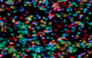
This means: the sequencer takes progressive digital photographs of the chip containing the sequencing reagent. These photos have differently coloured pixels which need to be told apart and assigned a specific colour value.

As can be seen, this (strongly magnified; the image is < 100 µm across!) image fragment is fuzzy and many of the dots overlap. This makes it hard to determine which colour to assign to which pixel (though more recent versions of the sequencing machine have improved focussing systems, and the image is consequently crisper).
Base calling
One such image is registered for each step of the sequencing process, yielding one image for each base of the fragments. For a fragment of length 75, that’d be 75 images.
Once you have analysed the images, you get colour spectra for each pixel across the images. The spectra for each pixel correspond to one sequence fragment (often called a “read”) and are considered separately. So for each fragment you get such a spectrum:

(This image is generated by an alternative sequencing process called Sanger sequencing but the principle is the same.)
Now you need to decide which base to assign for each position based on the signal (“base calling”). For most positions this is fairly easy but sometimes the signal overlaps or decays significantly. This has to be considered when deciding the base calling quality (i.e. which confidence you assign to your decision for a given base).
Doing this for each read yields up to billions of reads, each representing a short fragment of the original DNA that you sequenced.
Most bioinformatics analysis starts here; that is, the machines emit files containing the short sequence fragments. Now we need to make a sequence from them.
Read mapping and assembly
The key point that allows retrieving the original sequence from these small fragments is the fact that these fragments are (non-uniformly) randomly distributed over the genome, and they are overlapping.
The next step depends on whether you have a similar, already sequenced genome at hand. Often, this is the case. For instance, there is a high-quality “reference sequence” of the human genome and since all the genomic sequences of all humans are ~99.9% identical (depending on how you count), you can simply look where your reads align to the reference.
Read mapping
This is done to search for single changes between the reference and your currently studied genome, for example to detect mutations that lead to diseases.
So all you have to do is to map the reads back to their original location in the reference genome (in blue) and look for differences (such as base pair differences, insertions, deletions, inversions …).

Two points make this hard:
You have got billions (!) of reads, and the reference genome is often several gigabytes large. Even with the fastest thinkable implementation of string search, this would take prohibitively long.
The strings don’t match precisely. First of all, there are of course differences between the genomes – otherwise, you wouldn’t sequence the data at all, you’d already have it! Most of these differences are single base pair differences – SNPs (= single nucleotide polymorphisms) – but there are also larger variations that are much harder to deal with (and they are often ignored in this step).
Furthermore, the sequencing machines aren’t perfect. A lot of things influence the quality, first and foremost the quality of the sample preparation, and minute differences in the chemistry. All this leads to errors in the reads.
In summary, you need to find the position of billions of small strings in a larger string which is several gigabytes in size. All this data doesn’t even fit into a normal computer’s memory. And you need to account for mismatches between the reads and the genome.
Unfortunately, this still doesn’t yield the complete genome. The main reason is that some regions of the genome are highly repetitive and badly conserved, so that it’s impossible to map reads uniquely to such regions.
As a consequence, you instead end up with distinct, contiguous blocks (“contigs”) of mapped reads. Each contig is a sequence fragment, like reads, but much larger (and hopefully with less errors).
Assembly
Sometimes you want to sequence a new organism so you don’t have a reference sequence to map to. Instead, you need to do a de novo assembly. An assembly can also be used to piece contigs from a mapped reads together (but different algorithms are used).
Again we use the property of the reads that they overlap. If you find two fragments which look like this:
ACGTCGATCGCTAGCCGCATCAGCAAACAACACGCTACAGCCT
ATCCCCAAACAACACGCTACAGCCTGGCGGGGCATAGCACTGG
You can be quite certain that they overlap like this in the genome:
ACGTCGATCGCTAGCCGCATCAGCAAACAACACGCTACAGCCT
                  ATCCCCATTCAACACGCTA-AGCTTGGCGGGGCATACGCACTG
(Notice again that this isn’t a perfect match.)
So now, instead of searching for all the reads in a reference sequencing, you search for head-to-tail correspondences between reads in your collection of billions of reads.
If you compare the mapping of a read to searching a needle in a haystack (an often used analogy), then assembling reads is akin to comparing all the straws in the haystack to each other straw, and putting them in order of similarity.


