Basic sigmoidal curve looks like that: zero at $-\inf$ and one at $+\inf$. All in between should look like an integral of gaussian distribution. Take a look on this wiki page for more information. Now, the question, why sigmoidal curve is integral of gaussian function, I will leave out for now. My understanding is that gaussian distribution tells you how much system response will increase (say, efficiency of treatment) if you increase stimulus by $dx$. E.g., how much response changes when you go from $5$ to $5+dx$ versus from $10$ to $10+dt$.
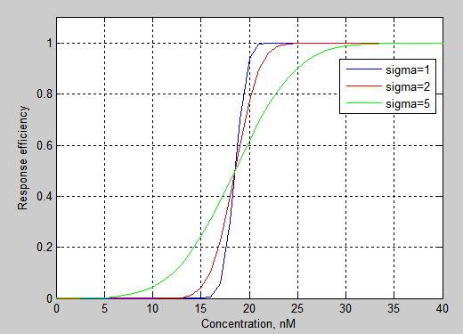
The problem, as you might realize, that gaussian distribution has two parameters: mean value and width of the function. When you construct your fit, frist one will be 19nM, but second, $\sigma$, is unknown from your question. What you don't know is how rapidly response changes when you increase concentration by little around your EC50. So all your sigmoidal plots will go through same point but with different slope, like that:

Without knowing second parameter, $\sigma$, it makes little sense to plot your sigmoidal curve. However, if you want to, this is MATLAB code. See that cumsum() function effectively integrates gaussian distribution rendering sigmoidal curve.
c = 0:100; % range of concentrations you test
sigma = 1; % unknown parameter
m = 19; % your EC50 19 nM
g = 1/(sigma*sqrt(2*pi))*exp(-((c - m).^2)/(2*sigma^2)); % gaussian
gs = cumsum(g);
plot(c, gs)
If you want, you can plot it with log-scale of X, using semilogx() instead of plot().
NB here I started with Gaussian function and its integral just as a wild guess. You real function might very well be something like $f(x)=\frac{1}{1+e^{-x}}$. "Sigmoid" function is just description of general shape, not mathematical definition.

