I think your issue is mainly with the interpretation of the isoclines.
If you assume this standard predator-prey model:
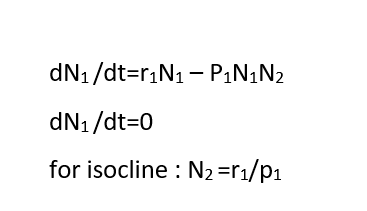
$$\frac{dN_1}{dt} = rN_1-pN_1N_2$$
$$\frac{dN_2}{dt} = apN_1N_2-mN_2$$
you get the isoclines:
$$ N_2 = \frac{r}{p} $$
$$ N_1 = \frac{m}{ap}$$
with the first isocline referring to prey and the second to predators. These isoclines mean that the population growth rate of prey and predators (respectively) will be zero exactly at these isoclines (as well as at the point N1=N2=0). Since the isoclines, for this partuicular model, are fixed values and not functions of N1 and/or N2 they will be strait lines. Also, in a sense, you should view the isoclines as the borderline case where population growth rate shifts between a positive and a negative value (ie a growing or a decreasing population). The isoclines are not giving you the population size of the prey at a certain predator population size (which you seem to be implying with "...why we are getting variable prey population on isocline for same value of predator population"), but the locations in the plane where the population growth rate (for either prey or predators) is zero.
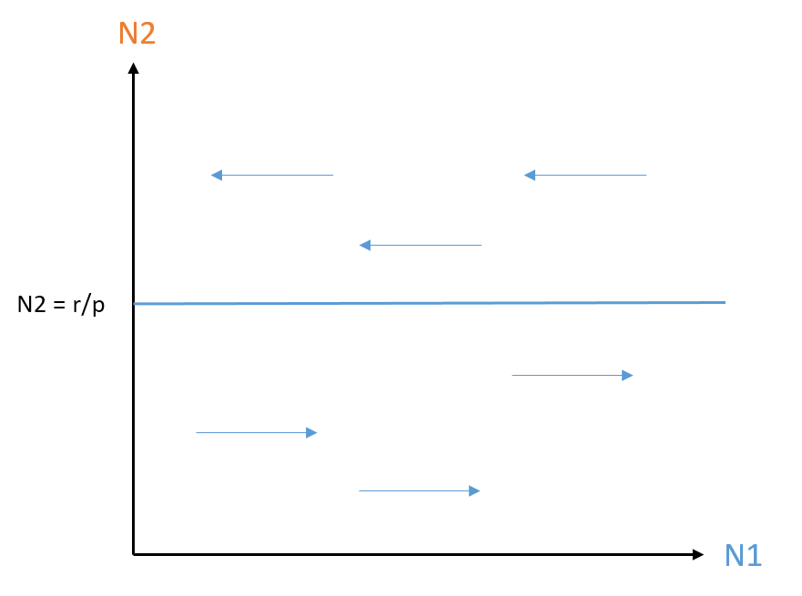
A graphical view of only the prey isocline (with some color coding) can be:

This means that the prey population (blue) is growing (arrows to the right) below the blue prey isocline, so there if a "flow" to the right there, while it is declining at predator population sizes above the isocline (arrows to the left). So basically, for all predator population sizes (N2) below isocline the prey population will grow, and for all N2 above the isocline the prey population will decline. In reality the rate of increase/decrease differs depending on how far from the isocline you are (so arrows should be of different lenghts), but to simplify the issue and to show the general principle I'm just showing the direction of flow here.
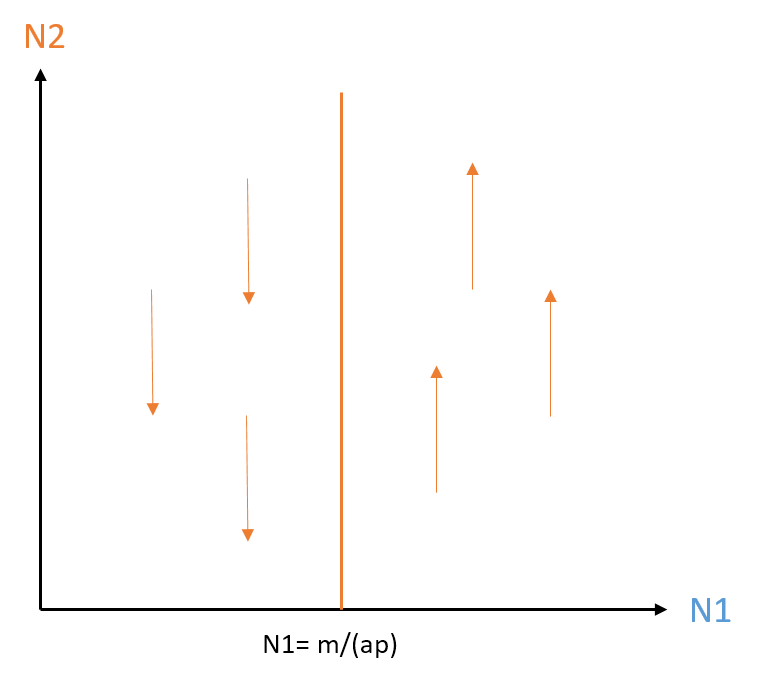
The same picture for the predator population is:

Here the predator population (orange) is declining to the left of the orange predator isocline (arrows down) because there is too little prey to sustain the population, and increasing to the right of the isocline (arrows up).
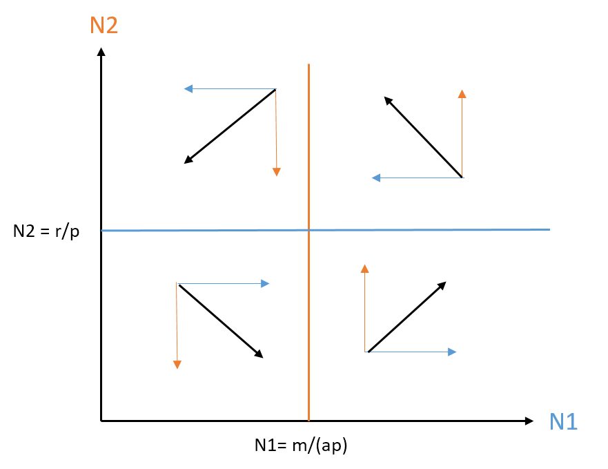
If you combine these you get this, with the black arrows showing the overall direction of the combined population trajectories:

I hope this clarifies the issue a bit. Otherwise, please comment and hightlight what parts you find unclear.
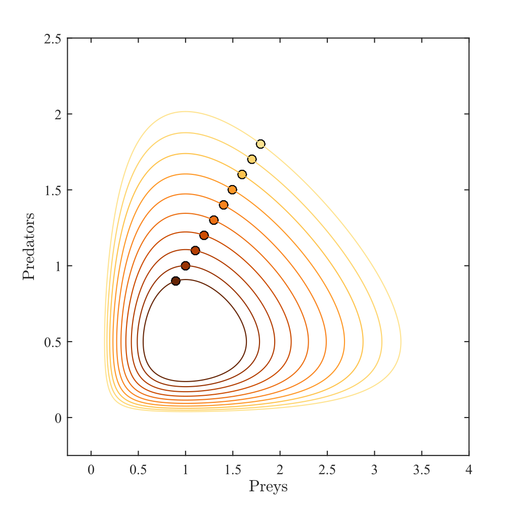
Also, the dynamics of this Lotka-Volterra model also means that populations that start exactly at the intersection of the isoclines (i.e. both N1 and N2 will lie at that point) will stay there, since that is an (unstable) equilibrium point. Populations that are started anywhere else in this plane (except for cases where N1 and/or N2 is zero), will follow an oscillating population trajectory, that will not change if there isn't any external pertubations (environmental changes, input/output through immigration/emmigration etc). Therefore, the combined trajectories of N1 and N2 will form an ellipse in the plane, until they are perturbed (by something outside the current model), when they will then settle at a new ellipsis. For examples of the ellipses, see this phase-plane graph from Wikipedia, with initial values as points:

However, also note that changing the model, i.e. to include a logistic component to the prey population, will completely change the population dynamics.
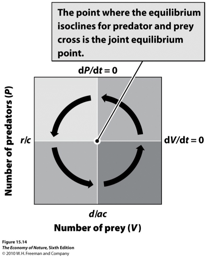 PS: I picked the graph image from the internet so the symbols are different. Sorry.
